ÜBUNGSSTUNDE 3 · ETH ZURICH · FS20 · analysis
Fundamentallimes, Teilfolgen und Limes superior Fundamentallimes, Teilfolgen, Häufungspunkte, Limes superior, Limes inferior, Cauchy Kriterium
SB
Steven Battilana Quant · ex-ETH
Nützliches: Fundamentallimes
lim n → ± ∞ ( 1 ± x n ) n = e ± x \lim\limits_{n \to \pm \infty} (1 \pm \frac{x}{n})^n = e^{\pm x} n → ± ∞ lim ( 1 ± n x ) n = e ± x lim n → ∞ ∧ f ( n ) → ∞ ( 1 + 1 f ( n ) ) f ( n ) = e \lim\limits_{n \to \infty \; \wedge \; f(n) \to \infty} (1 + \frac{1}{f(n)})^{f(n)} = e n → ∞ ∧ f ( n ) → ∞ lim ( 1 + f ( n ) 1 ) f ( n ) = e lim n → 0 ( 1 + n ) 1 n = e \lim\limits_{n \to 0} (1+n)^{\frac{1}{n}} = e n → 0 lim ( 1 + n ) n 1 = e lim n → 0 ( 1 + f ( n ) ) 1 f ( n ) = e \lim\limits_{n \to 0} (1+f(n))^{\frac{1}{f(n)}} = e n → 0 lim ( 1 + f ( n ) ) f ( n ) 1 = e Beispiel 1.1
Löse lim x → ∞ ( 1 − π x ) 2 x \lim\limits_{x \to \infty} (1-\frac{\pi}{x})^{2x} x → ∞ lim ( 1 − x π ) 2 x
Lösung anzeigen Lösung ausblenden lim x → ∞ ( 1 − π x ) 2 x = lim x → ∞ [ ( 1 + 1 − x π ) − x π ] − π x ⋅ 2 x = e − π x ⋅ 2 x = e − 2 π \begin{aligned}
\lim_{x \to \infty} (1-\frac{\pi}{x})^{2x} &= \lim_{x \to \infty} \left[ \left(1+\frac{1}{-\frac{x}{\pi}}\right)^{-\frac{x}{\pi}} \right]^{-\frac{\pi}{x} \cdot 2x}\\
&= e^{-\frac{\pi}{x} \cdot 2x}\\
&= e^{-2\pi}
\end{aligned} x → ∞ lim ( 1 − x π ) 2 x = x → ∞ lim [ ( 1 + − π x 1 ) − π x ] − x π ⋅ 2 x = e − x π ⋅ 2 x = e − 2 π
Beispiel 1.2
Löse lim x → 0 1 x log ( 1 + x 1 − x ) \lim\limits_{x \to 0} \frac{1}{x} \log(\frac{1+x}{1-x}) x → 0 lim x 1 log ( 1 − x 1 + x )
Lösung anzeigen Lösung ausblenden lim x → 0 1 x log ( 1 + x 1 − x ) = lim x → 0 log ( ( 1 + x 1 − x ) 1 x ) = lim x → 0 log ( ( 1 + x + x − x 1 − x ) 1 x ) = lim x → 0 log ( ( 1 − x + x + x 1 − x ) 1 x ) = lim x → 0 log ( ( 1 − x 1 − x + x + x 1 − x ) 1 x ) = lim x → 0 log ( ( 1 + 2 x 1 − x ) 1 x ) = lim x → 0 log ( [ ( 1 + 2 x 1 − x ) 1 − x 2 x ] 2 x 1 − x ⋅ 1 x ) = lim x → 0 log ( e 2 x 1 − x ⋅ 1 x ) = lim x → 0 log ( e 2 1 − x ) = log ( e 2 1 − 0 ) = log ( e 2 ) = 2 \begin{aligned}
\lim_{x \to 0} \frac{1}{x} \log \left( \frac{1+x}{1-x} \right) &= \lim_{x \to 0} \log \left(\left( \frac{1+x}{1-x}\right)^{\frac{1}{x}} \right)\\
&= \lim_{x \to 0} \log \left(\left( \frac{1+x + x-x}{1-x}\right)^{\frac{1}{x}} \right)\\
&= \lim_{x \to 0} \log \left(\left( \frac{1-x + x+x}{1-x}\right)^{\frac{1}{x}} \right)\\
&= \lim_{x \to 0} \log \left(\left( \frac{1-x}{1-x} + \frac{x+x}{1-x}\right)^{\frac{1}{x}} \right)\\
&= \lim_{x \to 0} \log \left(\left( 1 + \frac{2x}{1-x}\right)^{\frac{1}{x}} \right)\\
&= \lim_{x \to 0} \log \left(\left[\left( 1 + \frac{2x}{1-x}\right)^{\frac{1-x}{2x}} \right]^{\frac{2x}{1-x} \cdot \frac{1}{x}} \right)\\
&= \lim_{x \to 0} \log \left( e^{\frac{2x}{1-x} \cdot \frac{1}{x}} \right)\\
&= \lim_{x \to 0} \log \left( e^{\frac{2}{1-x}} \right)\\
&= \log \left( e^{\frac{2}{1-0}} \right)\\
&= \log \left( e^2 \right)\\
&= 2
\end{aligned} x → 0 lim x 1 log ( 1 − x 1 + x ) = x → 0 lim log ( ( 1 − x 1 + x ) x 1 ) = x → 0 lim log ( ( 1 − x 1 + x + x − x ) x 1 ) = x → 0 lim log ( ( 1 − x 1 − x + x + x ) x 1 ) = x → 0 lim log ( ( 1 − x 1 − x + 1 − x x + x ) x 1 ) = x → 0 lim log ( ( 1 + 1 − x 2 x ) x 1 ) = x → 0 lim log [ ( 1 + 1 − x 2 x ) 2 x 1 − x ] 1 − x 2 x ⋅ x 1 = x → 0 lim log ( e 1 − x 2 x ⋅ x 1 ) = x → 0 lim log ( e 1 − x 2 ) = log ( e 1 − 0 2 ) = log ( e 2 ) = 2
Cauchy Kriterium
Definition 2.1 Cauchy Folge
Eine Folge ( a n ) n ∈ N (a_n)_{n \in \mathbb{N}} ( a n ) n ∈ N Cauchy Folge , falls gilt:
∀ ε > 0 , ∃ N = N ( ε ) ∈ N : ∣ a n − a m ∣ < ε , ∀ n , m > N . \forall \varepsilon > 0, \; \exists N=N(\varepsilon) \in \mathbb{N}: \quad |a_n - a_m| < \varepsilon, \quad \forall n,m > N. ∀ ε > 0 , ∃ N = N ( ε ) ∈ N : ∣ a n − a m ∣ < ε , ∀ n , m > N .
Satz Cauchy Kriterium (3.5.1)
Sei ( a n ) ⊂ R (a_n) \subset \mathbb{R} ( a n ) ⊂ R
( a n ) (a_n) ( a n ) ( a n ) (a_n) ( a n )
Beispiel 2.1
Ist die Folge n − 1 2 n \frac{n-1}{2n} 2 n n − 1
Lösung anzeigen Lösung ausblenden Wir wählen ein (beliebig kleines) ε > 0 \varepsilon > 0 ε > 0 N N N m , n > N m,n > N m , n > N ∣ a n − a m ∣ < ε |a_n - a_m| < \varepsilon ∣ a n − a m ∣ < ε m ≥ n m \geq n m ≥ n n ≥ m n \geq m n ≥ m
∣ a n − a m ∣ = ∣ n − 1 2 n − m − 1 2 m ∣ = ∣ m ( n − 1 ) − n ( m − 1 ) 2 n m ∣ = ∣ n m − m − n m + n 2 n m ∣ = ∣ n − m 2 n m ∣ = ∣ 1 2 m − 1 2 n ∣ ≤ m ≥ n ∣ 1 2 n ∣ = ∣ 1 2 n ∣ < ! ε . ⇔ n > 1 2 ε ⇒ N = ⌈ 1 2 ε ⌉ \begin{aligned}
|a_n - a_m| &= \left| \frac{n-1}{2n} - \frac{m-1}{2m} \right|\\
&= \left| \frac{m(n-1) - n(m-1)}{2nm} \right|\\
&= \left| \frac{nm-m - nm+n}{2nm} \right|\\
&= \left| \frac{n-m}{2nm} \right|\\
&= \left| \frac{1}{2m} - \frac{1}{2n} \right|\\
&\stackrel{m \geq n}{\leq} \left| \frac{1}{2n} \right|\\
&= \left| \frac{1}{2n} \right|\\
&\stackrel{!}{<} \varepsilon.\\
&\Leftrightarrow \qquad n > \frac{1}{2 \varepsilon}\\
&\Rightarrow \qquad N = \left\lceil \frac{1}{2 \varepsilon} \right\rceil
\end{aligned} ∣ a n − a m ∣ = 2 n n − 1 − 2 m m − 1 = 2 nm m ( n − 1 ) − n ( m − 1 ) = 2 nm nm − m − nm + n = 2 nm n − m = 2 m 1 − 2 n 1 ≤ m ≥ n 2 n 1 = 2 n 1 < ! ε . ⇔ n > 2 ε 1 ⇒ N = ⌈ 2 ε 1 ⌉ Die Folge a n a_n a n R \mathbb{R} R
Teilfolgen, Häufungspunkte
Definition 3.1
Sei ( a n ) n ∈ N ⊂ R (a_n)_{n \in \mathbb{N}} \subset \mathbb{R} ( a n ) n ∈ N ⊂ R ℓ : N → Λ ⊂ N , n ↦ ℓ ( n ) \ell: \mathbb{N} \to \Lambda \subset \mathbb{N}, n \mapsto \ell(n) ℓ : N → Λ ⊂ N , n ↦ ℓ ( n ) ( a ℓ ( n ) ) (a_{\ell(n)}) ( a ℓ ( n ) ) ℓ ( n ) \ell(n) ℓ ( n ) a n a_n a n a n a_n a n
Beispiel 3.1
Sei ( a n ) n ∈ N = ( − 1 ) n (a_n)_{n \in \mathbb{N}} = (-1)^n ( a n ) n ∈ N = ( − 1 ) n R \mathbb{R} R
{ 1 , 1 , 1 , . . . } ( Λ = 2 N = { gerade Zahlen } ) { − 1 , − 1 , − 1 , . . . } ( Λ = 2 N + 1 = { ungerade Zahlen } ) \begin{aligned}
\{1, 1, 1, ...\} \qquad &( \Lambda = 2\mathbb{N} = \{\text{gerade Zahlen}\})\\
\{-1, -1, -1, ...\} \qquad &( \Lambda = 2\mathbb{N}+1 = \{\text{ungerade Zahlen}\})
\end{aligned} { 1 , 1 , 1 , ... } { − 1 , − 1 , − 1 , ... } ( Λ = 2 N = { gerade Zahlen }) ( Λ = 2 N + 1 = { ungerade Zahlen })
Definition 3.2
a ∈ R a \in \mathbb{R} a ∈ R ( a n ) n ∈ N (a_n)_{n \in \mathbb{N}} ( a n ) n ∈ N ( a n ) n ∈ N (a_n)_{n \in \mathbb{N}} ( a n ) n ∈ N a a a ( a ℓ ( n ) ) (a_{\ell(n)}) ( a ℓ ( n ) ) ( a ℓ ( n ) ) (a_{\ell(n)}) ( a ℓ ( n ) )
lim ℓ ( n ) → ∞ a ℓ ( n ) = a . \lim_{\ell(n) \to \infty} a_{\ell(n)} = a. ℓ ( n ) → ∞ lim a ℓ ( n ) = a .
Satz Bolzano-Weierstrass (3.4.1)
Jede beschränkte Folge ( a n ) n ∈ N (a_n)_{n \in \mathbb{N}} ( a n ) n ∈ N R \mathbb{R} R
Limes superior und Limes inferior
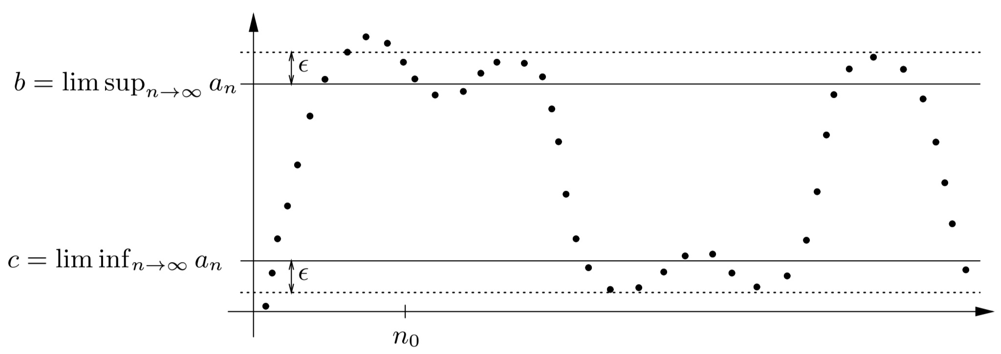
Definition 4.1 Limes superior und Limes inferior
Sei ( a n ) n ∈ N (a_n)_{n \in \mathbb{N}} ( a n ) n ∈ N
∃ M ∈ R , ∀ n ∈ N : ∣ a n ∣ < M . \exists M \in \mathbb{R}, \; \forall n \in \mathbb{N}: \quad |a_n| < M. ∃ M ∈ R , ∀ n ∈ N : ∣ a n ∣ < M . Für k ∈ N k \in \mathbb{N} k ∈ N
c k = inf n ≥ k a n ≤ sup n ≥ k a n = b k c_k = \inf_{n \geq k} a_n \leq \sup_{n \geq k} a_n = b_k c k = n ≥ k inf a n ≤ n ≥ k sup a n = b k Damit gilt
− M ≤ c 1 ≤ . . . ≤ c k ≤ c k + 1 ≤ b k + 1 ≤ b k ≤ . . . ≤ b 1 ≤ M , ∀ k ∈ N -M \leq c_1 \leq ... \leq c_k \leq c_{k+1} \leq b_{k+1} \leq b_k \leq ... \leq b_1 \leq M, \quad \forall k \in \mathbb{N} − M ≤ c 1 ≤ ... ≤ c k ≤ c k + 1 ≤ b k + 1 ≤ b k ≤ ... ≤ b 1 ≤ M , ∀ k ∈ N Mit dem Satz für monotone Konvergenz folgt die Existenz von
"Limes superior" : lim sup n → ∞ a n : = lim k → ∞ b k = b "Limes inferior" : lim inf n → ∞ a n : = lim k → ∞ c k = c \begin{aligned}
\text{"Limes superior"}: \qquad \limsup_{n \to \infty} a_n &:= \lim_{k \to \infty} b_k = b\\
\text{"Limes inferior"}: \qquad \liminf_{n \to \infty} a_n &:= \lim_{k \to \infty} c_k = c
\end{aligned} "Limes superior" : n → ∞ lim sup a n "Limes inferior" : n → ∞ lim inf a n := k → ∞ lim b k = b := k → ∞ lim c k = c und es gilt c ≤ b c \leq b c ≤ b
Satz
Es gilt
lim n → ∞ a n = a ⇔ lim sup n → ∞ a n = lim inf n → ∞ a n = lim n → ∞ a n = a . \lim_{n \to \infty} a_n = a \quad \Leftrightarrow \quad \limsup_{n \to \infty} a_n = \liminf_{n \to \infty} a_n = \lim_{n \to \infty} a_n = a. n → ∞ lim a n = a ⇔ n → ∞ lim sup a n = n → ∞ lim inf a n = n → ∞ lim a n = a .
Beispiel 4.1
Berechne lim sup a n \limsup a_n lim sup a n lim inf a n \liminf a_n lim inf a n
a n = ( − 1 ) n ⋅ n + 5 n = { ( − 1 ) ⋅ n + 5 n , f u ¨ r n ungerade n + 5 n , f u ¨ r n gerade \begin{aligned}
a_n &= (-1)^n \cdot \frac{n+5}{n}\\
&= \begin{cases}
(-1) \cdot \frac{n+5}{n}, & \text{für $n$ ungerade}\\
\frac{n+5}{n}, & \text{für $n$ gerade}
\end{cases}
\end{aligned} a n = ( − 1 ) n ⋅ n n + 5 = { ( − 1 ) ⋅ n n + 5 , n n + 5 , f u ¨ r n ungerade f u ¨ r n gerade Lösung anzeigen Lösung ausblenden Wir definieren c k : = ( − 1 ) ⋅ k + 5 k c_k := (-1) \cdot \frac{k+5}{k} c k := ( − 1 ) ⋅ k k + 5 b k : = k + 5 k b_k := \frac{k+5}{k} b k := k k + 5
lim inf n → ∞ a n = lim k → ∞ c k = − 1 lim inf n → ∞ ( − 1 ) n ⋅ n + 5 n = lim k → ∞ ( − 1 ) ⋅ k + 5 k = lim k → ∞ − k + 5 k = lim k → ∞ − k ( 1 + 5 k ) k = lim k → ∞ − 1 + 5 k 1 = lim k → ∞ − 1 − 5 k = − 1 − 0 = − 1 \begin{aligned}
\liminf_{n \to \infty} a_n &= \lim_{k \to \infty} c_k = -1\\
\liminf_{n \to \infty} (-1)^n \cdot \frac{n+5}{n} &= \lim_{k \to \infty} (-1) \cdot \frac{k+5}{k}\\
&= \lim_{k \to \infty} -\frac{k+5}{k}\\
&= \lim_{k \to \infty} -\frac{k(1+\frac{5}{k})}{k}\\
&= \lim_{k \to \infty} -\frac{1+\frac{5}{k}}{1}\\
&= \lim_{k \to \infty} -1-\frac{5}{k}\\
&= -1-0\\
&= -1
\end{aligned} n → ∞ lim inf a n n → ∞ lim inf ( − 1 ) n ⋅ n n + 5 = k → ∞ lim c k = − 1 = k → ∞ lim ( − 1 ) ⋅ k k + 5 = k → ∞ lim − k k + 5 = k → ∞ lim − k k ( 1 + k 5 ) = k → ∞ lim − 1 1 + k 5 = k → ∞ lim − 1 − k 5 = − 1 − 0 = − 1
lim sup n → ∞ a n = lim k → ∞ b k = 1 lim sup n → ∞ ( − 1 ) n ⋅ n + 5 n = lim k → ∞ k + 5 k = lim k → ∞ k ( 1 + 5 k ) k = lim k → ∞ 1 + 5 k 1 = 1 + 0 = 1 \begin{aligned}
\limsup_{n \to \infty} a_n &= \lim_{k \to \infty} b_k = 1\\
\limsup_{n \to \infty} \; (-1)^n \cdot \frac{n+5}{n} &= \lim_{k \to \infty} \frac{k+5}{k}\\
&= \lim_{k \to \infty} \frac{k(1+\frac{5}{k})}{k}\\
&= \lim_{k \to \infty} \frac{1+\frac{5}{k}}{1}\\
&= 1+0\\
&= 1
\end{aligned} n → ∞ lim sup a n n → ∞ lim sup ( − 1 ) n ⋅ n n + 5 = k → ∞ lim b k = 1 = k → ∞ lim k k + 5 = k → ∞ lim k k ( 1 + k 5 ) = k → ∞ lim 1 1 + k 5 = 1 + 0 = 1