In principle, the angle φ′ in the interval (0,2π] can be computed by first computing the angle in the interval (−π,π] as described above and then, only if it is negative, increasing it by 2π:
φ′={φ+2π,φ,φ<0otherwise.
Remark
As an alternative to arctan, φ can also be computed via sine and cosine:
The general case has m linear equations and n unknowns and forms a linear system. If
mmm>n, then the linear system is overdetermined (solvable numerically)<n, then the linear system is underdetermined (solvable analytically)=n, (solvable analytically)a11x1+a12x2+⋯+a1nxna21x1+a22x2+⋯+a2nxn⋮am1x1+am2x2+⋯+amnxn=b1=b2⋮=bm⎭⎬⎫⇒Ax=b
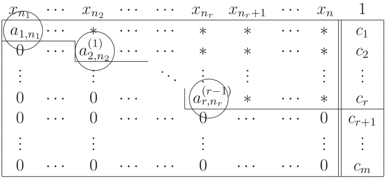
Using operations of type (I), (II), (III), bring (Ab) into the following form (row echelon form, i.e. it does not necessarily have to give the identity matrix!):
10⋱01x1⋮xn⇔(𝟙x), where 𝟙=^identity matrix
(I) Swap rows
(II) Add/subtract one row (equation) to/from another
(III) Multiply a row (equation) by k with k∈R∖{0}
This works best if you form the following ratio (we will need it again later!)
We choose x3=:s,s∈R∖{0} as a free parameter.
Back substitution in the 2nd row gives
ax2−3s=0⇔ax2=3s⇔x2=a3s
Back substitution in the 1st row gives
x1−s=0⇔x1=s
So we have already arrived at the solution for this case:
L=⎩⎨⎧sa3sss∈R∖{0},a=±2⎭⎬⎫
Case 2:x3=0
Then the 3rd row says nothing about a. So we have to fall back on the 2nd row.
ax2−3x3=0⇒ax2−3⋅0=0⇒ax2=0⇒a=0∨x2=0
(a) a = 0, x2=0:
We choose x2=t,t∈R∖{0} as a free parameter.
Back substitution in the 1st row gives x1=0. So we obtain the solution:
L=⎩⎨⎧0t0t∈R∖{0},a=0⎭⎬⎫
(b)x2=0:
Then the 1st row gives: x1=0
This case only yields the trivial solution 000 and can be excluded.
Altogether, we obtain nontrivial solutions for a∈{−2,0,2}.
Matrices and Vectors in Rn and Cn
Definition
The elements circled in the following figure are called pivot elements, or pivots for short.
Definitionpivoting
Pivot in the current column j, i.e. determine the index ip∈{j,j+1,...,m} with ∣aipj∣=i∈{j,j+1,...,m}max∣aij∣.
Definition
In the row echelon form (REF) of the system, the number r∈N of pivot elements is called the rank of the matrix A ∈Rm×n and of the linear system, i.e.
rank(A):=r=^# pivot elements.
Remark
Let the matrix A ∈Rm×n have rank r∈N, then
r≤min{m,n},
n−r=^#free parameters, where n is the number of unknowns.
Exampleon (ii)
m<n:
A=300010002−212−1⇝rank(A)=3
Here you can see that the rank cannot be more than 3, since the maximum possible number of pivot elements is 3.
m>n:
B=10000200−25−120⇝rank(B)=3
In this case the last row is linearly dependent, i.e. using the first three rows we can turn the last one into a zero row. So here, too, the maximum possible number of pivot elements is 3.
Now let us check the whole thing with Matlab.
We are in the Command Window:
% create the matrices A and B>> A = [2 -3 5; 1 0 2];>> B = [0 5; 1 1; -2 0];% carry out the multiplication>> A*Bans = -13 7 -4 5
Let us play a little more with Matlab so that you know all the functions you need to check for yourself whether you made a mistake.
Suppose you want to compute (AB)T=BTAT without transposing the matrices by hand:
% create the matrices A and B>> A = [2 -3 5; 1 0 2];>> B = [0 5; 1 1; -2 0];% carry out the multiplication>> (A*B)'ans = -13 -4 7 5>> B'*A'ans = -13 -4 7 5% create a 3-dim. identity matrix>> einheitsmatrix = eye(3);
Remark
The usual arithmetic rules (associativity, distributivity) hold for matrix multiplication. EXCEPT commutativity!!!(AB=BA) !!!!!
Definition
Let A be a realm×n matrix. The n×m matrix AT with (AT)ij=Aji is called the transpose of A.
Definition
Let A be a complexm×n matrix. The n×m matrix AH with AH=(A)T=AT is called the Hermitian or conjugate transpose of A.